The Extra Term

Abstract

In our previous note, The Geometry of Fluctuation, we established the geometric framework of multiplicative asset dynamics, leading to the formulation of Geometric Brownian Motion (GBM) and the identification of the −½σ²dt volatility correction. However, that derivation relied on the stochastic multiplication table and second-order Taylor expansions as algebraic axioms. This paper addresses the deep mathematical foundations underlying those rules, explaining precisely why classical deterministic calculus fails when applied to Brownian-driven processes. By examining the probabilistic and pathwise properties of Brownian motion, we explain why its infinite total variation causes the classical bounded-variation Riemann–Stieltjes framework to fail, while its quadratic variation determines the limiting second-order contribution. We analyze the heuristic scaling ΔW_t ~ √Δt and formalize it through the rigorous framework of quadratic variation, showing that [W]_t = t. We present Kiyosi Itô's 1951 Taylor-expansion proof to demonstrate why the second-order term survives in the continuous limit, thereby revealing how the deterministic quadratic variation of Brownian motion underlies the correction terms of Itô calculus.

Introduction

In our previous note, The Geometry of Fluctuation [1], we motivated the transition from additive to multiplicative price dynamics, resolving structural issues in asset pricing models by formulating price changes as percentage returns:

dS_t = \mu S_t dt + \sigma S_t dW_t

To solve this stochastic differential equation, we introduced the logarithmic transformation $X_t = \log S_t$ . Applying the non-classical chain rule known as Itô's Lemma, we arrived at the exact solution:

S_t = S_0 \exp\left( \left(\mu - \frac{1}{2}\sigma^2\right)t + \sigma W_t \right)

This solution contains the characteristic volatility correction term $-\frac{1}{2}\sigma^2 t$ , which arises as a direct mathematical consequence of the quadratic variation of Brownian paths.

While the utility of this correction is clear (it ensures that the expectation of the lognormal price process $\mathbb{E}[S_t]$ grows at the rate $\mu$ ), the derivation in The Geometry of Fluctuation accepted the stochastic differential multiplication rules, such as $(dW_t)^2 = dt$ , and the survival of the second-order Taylor term as algebraic assumptions. The goal of this technical note is to fill this conceptual gap. We address the fundamental mathematical question: why does classical calculus fail for Brownian-driven processes, and why must the second-order term be retained in the stochastic chain rule?

Rather than presenting the answer immediately, we begin with the rule encountered in the previous paper, $(dW_t)^2 = dt$ , and ask where it actually comes from. This rule represents a profound mathematical puzzle. In classical calculus, the square of a differential vanishes, $(dx)^2 = 0$ . How is it that squaring a random differential yields a deterministic time increment $dt$ ? The answer lies in the fine structure of Brownian paths, which forces a fundamental departure from classical integration. Because Brownian motion is highly oscillatory, its fine-scale jitter does not smooth away as the time partition is refined. Instead, this continuous fluctuation accumulates at a fixed, deterministic quadratic-variation rate, allowing second-order effects to persist in the continuous-time limit.

The Roughness of Brownian Motion

To understand why ordinary calculus fails, we must examine the pathwise behavior of standard Brownian motion $\{W_t\}_{t \geq 0}$ . A standard Brownian motion is a continuous, adapted process with $W_0 = 0$ almost surely, and independent, stationary, normally distributed increments: $W_{t+s} - W_t \sim \mathcal{N}(0, s)$ [2]. Despite their pathwise continuity, almost all sample paths of Brownian motion are highly pathological compared to the smooth functions analyzed in classical calculus.

For almost every path, the limit of the difference quotient:

\lim_{h \to 0} \frac{W_{t+h}(\omega) - W_t(\omega)}{h}

does not exist at any time $t \geq 0$ [2] [3]. Furthermore, for almost every path, the total variation defined by the supremum over all partitions:

V_t(W) = \sup_{\Pi} \sum_{k=1}^n |W_{t_k} - W_{t_{k-1}}|

is infinite on any finite interval $[0, t]$ [4].

This pathology motivates the need for a non-classical calculus. Because the paths exhibit an infinite number of fluctuations on any time scale and lack differentiability, the classical bounded-variation Riemann–Stieltjes framework fails generally for integrals of the form $\int_0^t H_s dW_s$ . Here, infinite total variation explains why the classical bounded-variation Riemann–Stieltjes framework fails, while quadratic variation determines the limiting second-order contribution.

Why the Second-Order Term Survives

We now examine the behavior of functions of Brownian motion. Consider a sufficiently smooth function $f(x)$ evaluated at $x = W_t$ . To understand how the process $f(W_t)$ evolves over a small time increment $\Delta t$ , we examine the difference $\Delta f = f(W_{t+\Delta t}) - f(W_t)$ .

Letting $\Delta W_t = W_{t+\Delta t} - W_t$ denote the Brownian increment, we perform a Taylor expansion of $f(W_{t+\Delta t})$ around $W_t$ :

f(W_{t+\Delta t}) - f(W_t) = f'(W_t)\Delta W_t + \frac{1}{2}f''(W_t)(\Delta W_t)^2 + \frac{1}{6}f'''(W_t)(\Delta W_t)^3 + \dots

In classical calculus, if we were expanding a function of a differentiable process $x_t$ , we would write the increment as $\Delta x_t = x'_{t} \Delta t + o(\Delta t)$ . The first-order term is proportional to $\Delta t$ , and the second-order term is proportional to $(\Delta x_t)^2 \approx (x'_t)^2 (\Delta t)^2$ . In the limit as $\Delta t \to 0$ , we discard $(\Delta x_t)^2$ and all higher-order terms because they vanish much faster than $\Delta t$ . The classical chain rule is the result of keeping only the first-order term.

This logic breaks down for Brownian motion. Because $W_{t+s} - W_t \sim \mathcal{N}(0, s)$ , the increment has standard deviation:

\text{std}(\Delta W_t) = \sqrt{\Delta t}

This provides the fundamental heuristic scaling relation for Brownian motion:

\Delta W_t \sim \sqrt{\Delta t}

This scaling is statistical, not a pathwise equality. It indicates that the typical size of a fluctuation over a small interval $\Delta t$ is of the order $\sqrt{\Delta t}$ .

Applying this statistical scaling to the terms in the Taylor expansion above, we find that $(\Delta W_t)^2 \sim \Delta t$ , while higher-order increments scale as $(\Delta t)^{k/2}$ for $k \geq 3$ . When we analyze the Taylor expansion under this scaling, we see that the first-order term $f'(W_t)\Delta W_t$ is of order $\sqrt{\Delta t}$ (representing the diffusion shock), while the second-order term $\frac{1}{2}f''(W_t)(\Delta W_t)^2$ is of order $\Delta t$ . Higher-order terms, when accumulated over a refining partition, have sums that vanish in the continuous-time limit as $\|\Pi\| \to 0$ under the regularity conditions used in the derivation.

Because $(\Delta W_t)^2$ scales as $\Delta t$ , the second-order term in the Taylor expansion is of the same order of magnitude as a standard time differential $dt$ . Consequently, this second-order term cannot be discarded; it must be retained alongside the first-order terms. The scaling argument explains why the second-order term can survive; quadratic variation explains what it converges to.

Quadratic Variation

To formalize the scaling intuition, we transition from heuristics to the mathematical framework of quadratic variation.

Definition

Let $\{X_t\}_{t \geq 0}$ be a continuous stochastic process. The quadratic variation process, denoted by $[X]_t$ , is defined as the limit in probability of the sum of squared increments when this limit exists, along a sequence of deterministic partitions $\Pi_n$ of $[0, t]$ whose mesh $\|\Pi_n\|$ tends to zero as $n \to \infty$ :

[X]_t = \text{p-lim}_{\|\Pi_n\| \to 0} \sum_{k=1}^{k_n} (X_{t_k} - X_{t_{k-1}})^2

where $\Pi_n = \{t_0, t_1, \dots, t_{k_n}\}$ is a partition of $[0, t]$ and $\|\Pi_n\|$ is its mesh.

For a classically differentiable function $g(t)$ with a continuous derivative, the quadratic variation is zero because the squared increments vanish as $\|\Pi\| \to 0$ . For Brownian motion, however, the quadratic variation is non-zero and deterministic.

Theorem

Let $\{W_t\}_{t \geq 0}$ be a standard Brownian motion. Then the quadratic variation over $[0, t]$ is:

[W]_t = t

Figure 1: Quadratic variation of a Brownian path under partition refinement on [0, 1].

Proof

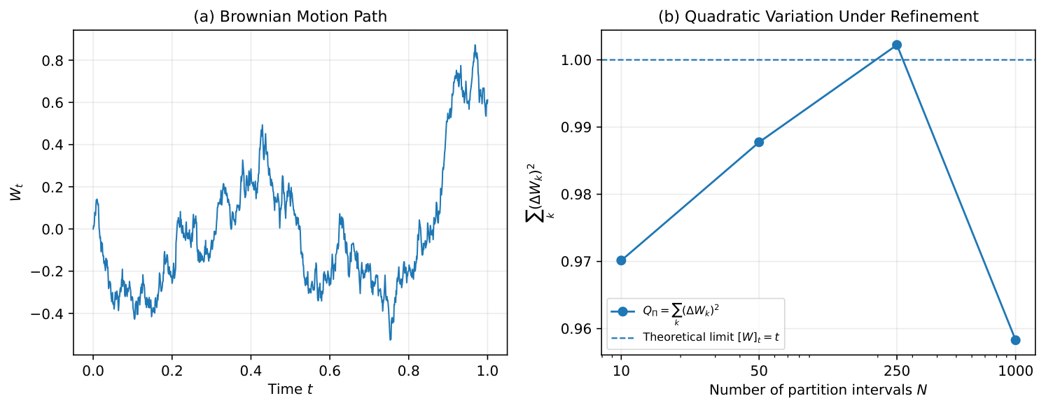
Let $\Pi = \{t_0, t_1, \dots, t_n\}$ be a partition of $[0, t]$ . Define the random variable:

Q_{\Pi} = \sum_{k=1}^n (W_{t_k} - W_{t_{k-1}})^2

Since the increments $W_{t_k} - W_{t_{k-1}}$ are independent and distributed as $\mathcal{N}(0, t_k - t_{k-1})$ , the expectation of $Q_{\Pi}$ is:

\mathbb{E}[Q_{\Pi}] = \sum_{k=1}^n (t_k - t_{k-1}) = t

Because the increments are independent and the variance of $Y^2$ for $Y \sim \mathcal{N}(0, \sigma^2)$ is $2\sigma^4$ , the variance of $Q_{\Pi}$ is:

\text{Var}(Q_{\Pi}) = 2 \sum_{k=1}^n (t_k - t_{k-1})^2 \leq 2 \|\Pi\| \sum_{k=1}^n (t_k - t_{k-1}) = 2 \|\Pi\| t

Taking the limit as the mesh of the partition $\|\Pi\| \to 0$ , we find that $\lim_{\|\Pi\| \to 0} \text{Var}(Q_{\Pi}) = 0$ .

This shows that the sum $Q_{\Pi}$ converges to $t$ in $L^2$ (mean-square) and hence in probability as the mesh $\|\Pi\| \to 0$ . The variance of the aggregate vanishes, so the accumulated squared increments concentrate around their deterministic mean $t$ . This limit provides the mathematical basis for the symbolic differential shorthand:

(dW_t)^2 = dt

This shorthand is a symbolic representation of convergence in probability, not an ordinary pathwise algebraic identity. It does not imply that the squared increment of Brownian motion over a small step is pointwise equal to the step size.

Similarly, the cross variation of Brownian motion with time vanishes. Although the total variation of Brownian motion is infinite almost surely, preventing the sum of absolute increments from converging to a finite limit, we can bound the expectation of the weighted increments. Specifically, the expectation of the weighted absolute increments behaves as:

\mathbb{E}\left[ \sum_{k=1}^n |W_{t_k} - W_{t_{k-1}}| (t_k - t_{k-1}) \right] = \sqrt{\frac{2}{\pi}} \sum_{k=1}^n (\Delta t_k)^{3/2} \leq \sqrt{\frac{2}{\pi}} t \sqrt{\|\Pi\|}

where $\Delta t_k = t_k - t_{k-1}$ . As $\|\Pi\| \to 0$ , this upper bound vanishes. Thus, the cross-term sums converge to zero in $L^1$ and therefore in probability, justifying the symbolic differential shorthand $dW_t dt = 0$ . By a similar argument, the quadratic variation of time with itself converges to zero, so that $(dt)^2 = 0$ . These limits explain why cross-multiplication terms involving $dt$ vanish in stochastic calculus, so, at second order, the Brownian quadratic-variation term is the only non-vanishing second-order contribution considered here. This quadratic variation mechanism underlies the correction terms of Itô calculus.

The Origin of Itô's Formula

We now turn to Itô's formula, whose detailed proof appears in Kiyosi Itô's 1951 paper, On a Formula Concerning Stochastic Differentials [5].

Let $f : [0, \infty) \times \mathbb{R} \to \mathbb{R}$ be a continuous function with continuous partial derivatives $f_t$ , $f_x$ , and $f_{xx}$ (i.e., $f \in C^{1,2}([0, \infty) \times \mathbb{R})$ ). We wish to express the differential of the process $f(t, W_t)$ .

Let us fix a time $t > 0$ and consider a partition $\Pi = \{t_0, t_1, \dots, t_m\}$ of $[0, t]$ with $0 = t_0 < t_1 < \dots < t_m = t$ . We can write the difference $f(t, W_t) - f(0, W_0)$ as a telescoping sum:

f(t, W_t) - f(0, W_0) = \sum_{k=1}^m \left[ f(t_k, W_{t_k}) - f(t_{k-1}, W_{t_{k-1}}) \right]

We decompose each increment in the sum as:

f(t_k, W_{t_k}) - f(t_{k-1}, W_{t_{k-1}}) = [f(t_k, W_{t_k}) - f(t_{k-1}, W_{t_k})] + [f(t_{k-1}, W_{t_k}) - f(t_{k-1}, W_{t_{k-1}})]

Applying the Mean Value Theorem to the first term (the time increment) and a second-order Taylor expansion to the second term (the space increment), we obtain:

\begin{align} f(t_k, W_{t_k}) - f(t_{k-1}, W_{t_{k-1}}) ={}& f_t(\tau_k, W_{t_k})(t_k - t_{k-1}) \nonumber \\ &+ f_x(t_{k-1}, W_{t_{k-1}})(W_{t_k} - W_{t_{k-1}}) \nonumber \\ &+ \frac{1}{2} f_{xx}(t_{k-1}, \eta_k)(W_{t_k} - W_{t_{k-1}})^2 \end{align}

where $t_{k-1} \leq \tau_k \leq t_k$ and $\eta_k$ is an intermediate point between $W_{t_{k-1}}$ and $W_{t_k}$ [2] [5].

Substituting this back into the telescoping sum above, we partition the expression into three distinct sums:

f(t, W_t) - f(0, W_0) = S_1(\Pi) + S_2(\Pi) + S_3(\Pi)

where:

\begin{align} S_1(\Pi) &= \sum_{k=1}^m f_t(\tau_k, W_{t_k})(t_k - t_{k-1}) \\ S_2(\Pi) &= \sum_{k=1}^m f_x(t_{k-1}, W_{t_{k-1}})(W_{t_k} - W_{t_{k-1}}) \\ S_3(\Pi) &= \frac{1}{2} \sum_{k=1}^m f_{xx}(t_{k-1}, \eta_k)(W_{t_k} - W_{t_{k-1}})^2 \end{align}

Before taking limits, we identify the role of each sum. The first sum, $S_1(\Pi)$ , represents the accumulated time contribution. The second sum, $S_2(\Pi)$ , is the approximating sum for the stochastic spatial integral. The third sum, $S_3(\Pi)$ , contains the second-order spatial derivative weighted by the squared Brownian increments. This third sum is the central mathematical object of study.

We analyze the convergence of these sums as $\|\Pi\| \to 0$ :

The time component $S_1(\Pi)$ is a standard Riemann sum. Since $f_t$ and the paths of $W_t$ are continuous, it converges pathwise to the ordinary Lebesgue integral:
$S_1(\Pi) \to \int_0^t f_t(s, W_s) ds \quad \text{almost surely}$
The spatial component $S_2(\Pi)$ is evaluated at the left-endpoint of each subinterval. This ensures that the integrand is adapted (non-anticipating). Assuming the standard square-integrability condition $\mathbb{E}\left[ \int_0^t f_x(s, W_s)^2 ds \right] < \infty$ , as $\|\Pi\| \to 0$ the left-endpoint sums $S_2(\Pi)$ converge in the $L^2$ sense (and therefore in probability) to the stochastic integral:
$S_2(\Pi) \to \int_0^t f_x(s, W_s) dW_s$
defining the standard Itô stochastic integral.
To establish the convergence of the second-order sum $S_3(\Pi)$ , we assume standard regularity and local integrability conditions on the derivatives. Specifically, we assume the square-integrability condition $\sup_{s \leq t} \mathbb{E}[f_{xx}(s, W_s)^2] < \infty$ , which can be extended to the general case via a standard localization argument. Since Brownian paths are bounded almost surely on finite intervals, standard localization allows us to work on a compact spatial region $[-M, M]$ where $f_{xx}$ is uniformly continuous.

We compare the sum $S_3(\Pi)$ to the left-endpoint Riemann sum:

S_4(\Pi) = \frac{1}{2} \sum_{k=1}^m f_{xx}(t_{k-1}, W_{t_{k-1}})(W_{t_k} - W_{t_{k-1}})^2

Due to the uniform continuity of $f_{xx}$ on the compact region, the difference between $S_3(\Pi)$ and $S_4(\Pi)$ converges to zero in probability. We then show that $S_4(\Pi)$ converges in probability to $\frac{1}{2} \int_0^t f_{xx}(s, W_s) ds$ by showing that the variance of the difference:

D_{\Pi} = \sum_{k=1}^m g_{k-1} \left[ (W_{t_k} - W_{t_{k-1}})^2 - (t_k - t_{k-1}) \right]

where $g_{k-1} = f_{xx}(t_{k-1}, W_{t_{k-1}})$ , vanishes as $\|\Pi\| \to 0$ . The variance is bounded by:

\text{Var}(D_{\Pi}) = 2 \sum_{k=1}^m \mathbb{E}[g_{k-1}^2] (t_k - t_{k-1})^2 \leq 2 \|\Pi\| t \sup_{s \leq t} \mathbb{E}[f_{xx}(s, W_s)^2]

Under the square-integrability condition $\sup_{s \leq t} \mathbb{E}[f_{xx}(s, W_s)^2] < \infty$ , taking the limit as $\|\Pi\| \to 0$ shows that $\text{Var}(D_{\Pi}) \to 0$ . Thus, $D_{\Pi} \to 0$ in $L^2$ and therefore in probability.

Refining the spatial evaluations over our partition and taking limits, we obtain:

S_3(\Pi) \to \frac{1}{2} \int_0^t f_{xx}(s, W_s) ds \quad \text{in probability}

Combining these limits, we obtain the integral form of Itô's Lemma:

f(t, W_t) - f(0, W_0) = \int_0^t f_t(s, W_s) ds + \int_0^t f_x(s, W_s) dW_s + \frac{1}{2} \int_0^t f_{xx}(s, W_s) ds

In differential notation, this is written as:

df(t, W_t) = f_t(t, W_t) dt + f_x(t, W_t) dW_t + \frac{1}{2} f_{xx}(t, W_t) dt

The derivation reveals that the $\frac{1}{2}$ coefficient is the coefficient of the second derivative in the Taylor expansion, surviving because the sum of squared Brownian increments converges in probability to the elapsed time.

The Correction Revisited

We now apply the rigorous Itô formula to resolve the logarithmic transformation of Geometric Brownian Motion presented in our previous paper [1].

Recall that Geometric Brownian Motion is governed by the SDE:

dS_t = \mu S_t dt + \sigma S_t dW_t

To find the dynamics of $X_t = \log S_t$ , we define the function $f(t, s) = \log s$ . We compute the partial derivatives of $f$ : $f_t = 0$ , $f_s = 1/s$ , and $f_{ss} = -1/s^2$ . Applying Itô's formula, we write:

d(\log S_t) = \frac{1}{S_t} dS_t + \frac{1}{2}\left( -\frac{1}{S_t^2} \right) d[S]_t

To evaluate this expression, we must determine the quadratic variation of the price process, $[S]_t$ . Rather than relying on symbolic manipulation, we appeal to the standard quadratic variation result for Itô processes, as established in Karatzas & Shreve [2], Chung & Williams [4], and Shreve [6]. An Itô process consists of a finite-variation drift component and a continuous local martingale diffusion component. The finite-variation drift component contributes zero to the quadratic variation, while the diffusion component contributes:

[S]_t = \int_0^t \sigma^2 S_u^2 d[W]_u = \int_0^t \sigma^2 S_u^2 du

Here we explicitly state that while the Brownian quadratic variation $[W]_t = t$ is deterministic, the price-process quadratic variation $[S]_t = \int_0^t \sigma^2 S_u^2 du$ is generally random, as it depends on the stochastic paths of the asset price itself.

At the partition level, this results from the same Brownian quadratic variation mechanism established in the previous section. Specifically, when we sum the squared increments of $S_t$ over a partition, the squared drift increments are $O((\Delta t)^2)$ and the drift-diffusion cross-terms are $O((\Delta t)^{3/2})$ , so both vanish after summation as $\|\Pi\| \to 0$ . The squared diffusion increments, on the other hand, contain $(W_{t_k} - W_{t_{k-1}})^2$ , which concentrates around $\Delta t_k$ with vanishing variance, yielding the quadratic-variation integral $\int_0^t \sigma^2 S_u^2 du$ in the limit. Thus, in differential notation, we write $d[S]_t = \sigma^2 S_t^2 dt$ .

Substituting $dS_t$ and $d[S]_t$ back into the expanded differential above (using $d[S]_t = \sigma^2 S_t^2 dt$ ):

\begin{align} d(\log S_t) &= \frac{1}{S_t} (\mu S_t dt + \sigma S_t dW_t) - \frac{1}{2 S_t^2} \sigma^2 S_t^2 dt \\ &= (\mu dt + \sigma dW_t) - \frac{1}{2} \sigma^2 dt \nonumber \end{align}

Grouping the deterministic time terms, we obtain the SDE for the log-price:

d(\log S_t) = \left( \mu - \frac{1}{2}\sigma^2 \right) dt + \sigma dW_t

Thus the log-price follows a Brownian motion with drift $\mu - \frac{1}{2}\sigma^2$ and diffusion coefficient $\sigma$ . Integrating both sides from 0 to $t$ yields:

\log S_t - \log S_0 = \left( \mu - \frac{1}{2}\sigma^2 \right) t + \sigma W_t

Exponentiating both sides results in the closed-form solution:

S_t = S_0 \exp\left( \left( \mu - \frac{1}{2}\sigma^2 \right) t + \sigma W_t \right)

which is exactly the closed-form solution stated in the introduction.

This derivation reveals the exact origin of the $-\frac{1}{2}\sigma^2 dt$ correction term. It is the direct product of:

The $\frac{1}{2}$ coefficient from the second-order term of the Taylor expansion of the logarithmic function.
The negative sign arising from the second derivative of the logarithm, $f_{ss}(s) = -1/s^2$ , reflecting the concavity of the log transformation.
The quadratic variation of the price process, $d[S]_t = \sigma^2 S_t^2 dt$ .

Because Brownian paths possess non-zero quadratic variation, the concave nature of the logarithmic function acts to reduce the drift of the log-transformed process.

The Extra Term

The extra term was already present in the Taylor expansion. What Brownian motion changes is whether that term disappears. In classical calculus, differentiable or $C^1$ paths have increments of order $\Delta t$ . Consequently, their squared increments are of order $O(\Delta t^2)$ , which vanish in the continuous limit and allow us to discard all but the first-order terms. For Brownian motion, however, the statistical scaling of increments is of order $O(\sqrt{\Delta t})$ , which means that the squared spatial increments scale as $O(\Delta t)$ and persist in the limit.

Itô's Lemma is the mathematical formulation of this persistence. The extra term arises directly from the second-order spatial derivative in the Taylor expansion. This second-order term is preserved because Brownian paths accumulate quadratic variation at a deterministic rate of one per unit time.

The master formula of this non-classical calculus, whose detailed proof we have examined, is expressed as:

\boxed{df(t, W_t) = f_t dt + f_x dW_t + \frac{1}{2} f_{xx} dt}

This extra term is the second-order Taylor contribution preserved by Brownian quadratic variation.

References

Pradhan, Sourabh. "The Geometry of Fluctuation." 2026.
Karatzas, Ioannis, and Steven Shreve. Brownian Motion and Stochastic Calculus. 2nd ed. Graduate Texts in Mathematics 113. Springer, 1991.
Øksendal, Bernt. Stochastic Differential Equations: An Introduction with Applications. 6th ed. Springer, 2003.
Chung, Kai Lai, and Ruth J. Williams. Introduction to Stochastic Integration. 2nd ed. Birkhäuser, 1990.
Itô, Kiyosi. "On a Formula Concerning Stochastic Differentials." Nagoya Mathematical Journal 3 (1951): 55–65.
Shreve, Steven E. Stochastic Calculus for Finance II: Continuous-Time Models. Springer, 2004.