The Geometry of Fluctuation

Abstract

This technical note examines why financial price movements are better modeled as relative rather than absolute changes. While arithmetic Brownian motion captures continuous fluctuations, its absolute, additive structure fails to reflect the proportional scaling of speculative returns and permits negative asset prices. We resolve these anomalies by modeling price changes as percentage returns, leading to the formulation of Geometric Brownian Motion. Using Itô's stochastic calculus, we derive the closed-form solution to this process and explain the origin of the -σ²/2 correction. We examine the resulting lognormal distribution, the structural positivity of asset prices, and discuss the model's role in continuous-time finance, concluding with a concise analysis of its limitations.

From Additive Limits to Relative Movements

In the study of random fluctuations, Brownian motion was constructed as the continuous-time limit of a scaled random walk. This continuous-time process, standard Brownian motion $W_t$ , provides a mathematically rigorous representation of continuous fluctuations with independent, stationary Gaussian increments [6]. In his 1900 doctoral thesis, Louis Bachelier utilized this framework to model speculative prices, proposing what is now termed arithmetic Brownian motion [1]:

S_t = S_0 + \mu t + \sigma W_t

Here, the asset price $S_t$ is modeled as a balance between a deterministic drift parameter $\mu$ and a random fluctuation term scaled by the volatility coefficient $\sigma$ .

Bachelier's model was a genuine breakthrough, but it has one structural problem. Under arithmetic Brownian motion, price changes are absolute and additive. Over a small time interval $\Delta t$ , the price increment is given by:

\Delta S_t = S_{t+\Delta t} - S_t = \mu \Delta t + \sigma \Delta W_t

Because the price increment $\Delta S_t$ is independent of the current price level $S_t$ , the model treats a $5 price movement on a $10 asset with the exact same probability as a $5 movement on a $500 asset. In competitive markets, however, market participants do not evaluate absolute changes in isolation; they evaluate percentage returns. A $5 decline on a $10 stock represents a 50% loss of capital, whereas a $5 decline on a $500 stock is a negligible 1% fluctuation. Absolute changes do not scale with the level of the system.

A secondary structural flaw of this additive structure is that the price $S_t$ can drop below zero. Because the absolute increments are normally distributed, the probability that the price will be negative at time $t$ is strictly positive:

P(S_t < 0) = \Phi\left( -\frac{S_0 + \mu t}{\sigma \sqrt{t}} \right) > 0

where $\Phi$ represents the cumulative standard normal distribution function. For long-term forecasts or in regimes of high volatility, this probability can become substantial. Real-world stock and equity prices cannot fall below zero; a negative price lacks physical meaning in market exchange. The model treats a $20 decline and a $20 increase as equally admissible outcomes, even when the decline would take the price below zero. This motivates a model where price changes are relative rather than absolute, and where prices remain positive.

Multiplicative Dynamics

To construct a model that reflects the relative nature of prices, we must formulate price changes as percentage returns. Over a small time interval $\Delta t$ , we expect the change in the price, $\Delta S_t$ , to scale proportionally with the current price level, $S_t$ . We can write this percentage return as an approximate small-time relation:

\frac{\Delta S_t}{S_t} \approx \mu \Delta t + \sigma \Delta W_t

This is a discrete-time approximation where the percentage return has constant drift and volatility parameters. Passing to the continuous-time limit, the dynamics of the price are governed by the stochastic differential equation:

dS_t = \mu S_t dt + \sigma S_t dW_t

This SDE defines Geometric Brownian Motion. Here, both the deterministic drift and the random diffusion scale with the current price level. If the price increases, its fluctuations scale up proportionally; if the price falls, its fluctuations contract.

For an asset initialized at $S_0 > 0$ , the continuous-time process $S_t$ remains strictly positive for every finite $t$ , meaning that zero is inaccessible in finite time. If the process were instead initialized at zero ( $S_0 = 0$ ), both the drift and the diffusion coefficients would vanish, rendering zero an absorbing state of the stochastic differential equation.

When Ordinary Calculus Fails

The transition from an additive model to a multiplicative model alters the mathematics required to solve the process. If we apply the rules of ordinary calculus to integrate this SDE, we can divide both sides by $S_t$ to isolate the terms:

\frac{dS_t}{S_t} = \mu dt + \sigma dW_t

Integrating both sides from $0$ to $t$ yields:

\int_0^t \frac{dS_s}{S_s} = \int_0^t \mu ds + \int_0^t \sigma dW_s

Under standard calculus, the integral of $1/x$ is the natural logarithm, which would suggest:

\log S_t - \log S_0 = \mu t + \sigma W_t

Exponentiating both sides would then give the candidate solution:

S_t = S_0 \exp(\mu t + \sigma W_t)

This candidate solution, however, is mathematically incorrect. The failure of ordinary calculus is a consequence of the path properties of standard Brownian motion. Standard Brownian motion is continuous everywhere but differentiable nowhere, and its sample paths possess infinite total variation. Brownian motion accumulates quadratic variation at a deterministic rate of one per unit time [6]. Path-by-path, the quadratic variation over the interval $[0, t]$ is:

[W, W]_t = \lim_{\|\Pi\| \to 0} \sum_{j=0}^{n-1} (W_{t_{j+1}} - W_{t_j})^2 = t \quad \text{almost surely}

Informally, this is expressed through the multiplication rule:

(dW_t)^2 = dt

Because the squared differential $(dW_t)^2$ is of order $dt$ , we cannot discard second-order terms when expanding functions of a stochastic process. When we Taylor-expand a function $f(S_t)$ , the second-order derivative term remains in the limit and introduces a systematic drift correction. To evaluate the logarithmic transformation correctly, we must employ the stochastic counterpart of the chain rule, known as Itô's lemma.

The Logarithmic Transformation and Solution

To solve the stochastic differential equation for Geometric Brownian Motion, we seek a transformation that removes the state dependence from the coefficients. We define the transformed process $X_t = \log S_t$ , which corresponds to the function $f(S_t) = \log S_t$ . The logarithm is the natural transformation for this multiplicative system because its derivative, $f'(S_t) = 1/S_t$ , naturally cancels out the state-dependent factor $S_t$ in the drift and diffusion coefficients of Geometric Brownian Motion.

We state Itô's lemma for a twice-differentiable function $f(S_t)$ of a stochastic process:

df(S_t) = f'(S_t) dS_t + \frac{1}{2} f''(S_t) (dS_t)^2

To apply this lemma, we compute the first and second derivatives of our function $f(S_t) = \log S_t$ with respect to the state variable:

f'(S_t) = \frac{1}{S_t}, \quad f''(S_t) = -\frac{1}{S_t^2}

Substituting these derivatives into Itô's lemma yields:

d(\log S_t) = \frac{1}{S_t} dS_t - \frac{1}{2S_t^2} (dS_t)^2

Next, we evaluate the squared price differential $(dS_t)^2$ . Utilizing the SDE and the stochastic multiplication rules ( $(dW_t)^2 = dt$ , $dt^2 = 0$ , and $dt\, dW_t = 0$ ), we have:

(dS_t)^2 = (\mu S_t dt + \sigma S_t dW_t)^2 = \mu^2 S_t^2 (dt)^2 + 2\mu\sigma S_t^2 dt\, dW_t + \sigma^2 S_t^2 (dW_t)^2

Applying the multiplication rules, the first two terms vanish, and the final term reduces to:

(dS_t)^2 = \sigma^2 S_t^2 dt

Substituting the expressions for $dS_t$ and $(dS_t)^2$ back into our expanded differential yields:

d(\log S_t) = \frac{1}{S_t} (\mu S_t dt + \sigma S_t dW_t) - \frac{1}{2S_t^2} (\sigma^2 S_t^2 dt)

We can distribute $1/S_t$ and $1/S_t^2$ , which simplifies the expression to:

d(\log S_t) = \mu dt + \sigma dW_t - \frac{1}{2} \sigma^2 dt

Grouping the deterministic drift terms together, we arrive at:

d(\log S_t) = \left( \mu - \frac{\sigma^2}{2} \right) dt + \sigma dW_t

The logarithmic transformation removes $S_t$ entirely from the drift and diffusion coefficients. The process governing $d(\log S_t)$ is an arithmetic Brownian motion with a modified constant drift coefficient of $(\mu - \sigma^2/2)$ . Because the drift and diffusion coefficients of this transformed process are constant, the remaining integration can be handled directly using standard calculus:

\log S_t - \log S_0 = \left( \mu - \frac{\sigma^2}{2} \right) t + \sigma W_t

Exponentiating both sides yields the exact, closed-form solution for Geometric Brownian Motion:

S_t = S_0 \exp\left[ \left( \mu - \frac{\sigma^2}{2} \right) t + \sigma W_t \right]

The Volatility Correction and Lognormal Prices

The appearance of the $-\sigma^2/2$ term in the exponent is a direct consequence of the quadratic variation of Brownian paths. We can understand its financial meaning by examining the expected value and the median of the asset price distribution.

Because $W_t$ is normally distributed with mean zero and variance $t$ , the term $e^{\sigma W_t}$ is a lognormal random variable. Using the moment-generating function of a normal distribution, the expectation is given by:

\mathbb{E}\left[ e^{\sigma W_t} \right] = e^{\frac{1}{2}\sigma^2 t}

Taking the expectation of our closed-form solution, we find:

\mathbb{E}[S_t] = \mathbb{E}\left[ S_0 \exp\left[ \left( \mu - \frac{\sigma^2}{2} \right) t + \sigma W_t \right] \right] = S_0 \exp\left[ \left( \mu - \frac{\sigma^2}{2} \right) t \right] \mathbb{E}\left[ e^{\sigma W_t} \right]

Substituting this expectation yields:

\mathbb{E}[S_t] = S_0 \exp\left[ \left( \mu - \frac{\sigma^2}{2} \right) t \right] \exp\left( \frac{1}{2} \sigma^2 t \right) = S_0 e^{\mu t}

The expected price of the asset grows at rate $\mu$ . Volatility $\sigma$ has no effect on that growth rate.

The realized path of an individual stock, however, is not described by its expected price. Since $W_t \sim N(0,t)$ , its median is zero. The median of the stock price $S_t$ is therefore:

\text{Median}(S_t) = S_0 \exp\left[ \left( \mu - \frac{\sigma^2}{2} \right) t \right]

Since $\sigma^2 > 0$ , the median of the distribution is strictly less than the expected price. This inequality reflects the right-skewness of the lognormal distribution. The $-\sigma^2/2$ correction term lowers the drift of the log-price, so the median price grows at a lower rate than the expected price. The convexity of the exponential function magnifies large positive shocks, which pulls the expected price upward. As a result, more than half of realized prices at any fixed time $t$ lie below the expected price. Figure 1 illustrates this divergence directly.

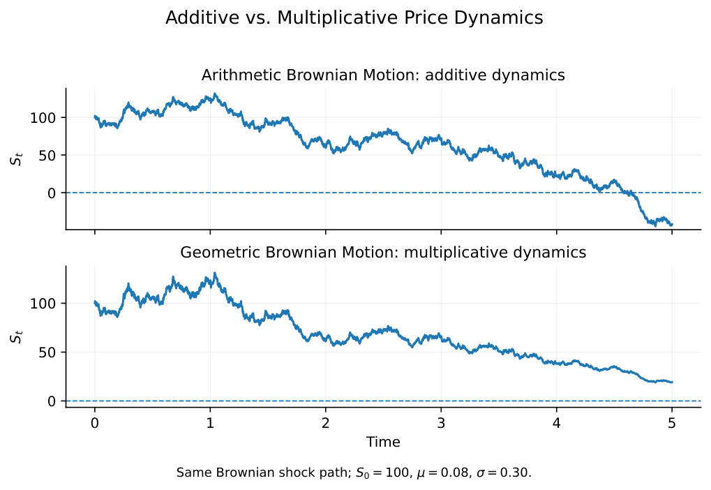
Sample paths of ABM and GBM driven by the same Brownian shocks — Figure 1: Sample paths of Arithmetic Brownian Motion (ABM) and Geometric Brownian Motion (GBM) driven by the same Brownian shocks. The ABM path crosses below zero, while GBM remains strictly positive. Parameters: S₀ = 100, μ = 0.08, σ = 0.30.

Over long horizons, this skewness has a sharp asymptotic consequence. For any $\sigma > 0$ , the normalized price $S_t / \mathbb{E}[S_t]$ converges to zero almost surely as $t \to \infty$ . Furthermore, if the volatility is sufficiently large such that $\sigma^2 > 2\mu$ , the stock price $S_t$ itself converges to zero almost surely as $t \to \infty$ , even though the expected price $\mathbb{E}[S_t] = S_0 e^{\mu t}$ grows exponentially to infinity when $\mu > 0$ .

Because $S_t$ is expressed as the exponential of a real-valued normal random variable, the price remains strictly positive for any finite time $t$ , provided the initial price $S_0$ is positive, ensuring that the process never reaches or crosses zero in finite time.

Historical and Financial Context

In 1959, M.F.M. Osborne modified Bachelier's model by considering not absolute price changes but their logarithm, drawing on the physics of particle motion to relate stock market variations to Brownian motion in the logarithm of price [4]. In 1965, Paul Samuelson formalized this into geometric Brownian motion and applied it to warrant pricing [5]. Black, Scholes, and Merton built their 1973 option-pricing models on this multiplicative framework [2, 3]. Their work showed how such continuous-time price dynamics could be combined with no-arbitrage arguments to value derivatives.

Limitations of the Geometric Model

Despite its mathematical tractability and widespread adoption, Geometric Brownian Motion is an idealized representation of financial markets. Empirical observations of speculative prices reveal several critical limitations:

Constant Volatility: The model assumes that the volatility parameter $\sigma$ is constant. In real-world markets, volatility is highly dynamic, fluctuating over time and clustering in regimes of high and low intensity.
Continuous Paths: The sample paths of Brownian motion are continuous. Financial asset prices, however, frequently exhibit discrete, discontinuous jumps in response to news and macroeconomic events.
Heavy Tails: The normal distribution of log returns under GBM underestimates the probability of extreme market movements. Empirical return distributions possess excess kurtosis (heavy tails), meaning that extreme returns occur more frequently than predicted by a lognormal model.
Parameter Instability: The drift parameter $\mu$ and volatility $\sigma$ are assumed to remain constant, but real-world markets undergo structural breaks, shifting across different macroeconomic and regulatory regimes.

Conclusion

Geometric Brownian Motion addresses the scaling and negativity issues of additive models by formulating price changes as percentage returns. This provides a tractable, positive price process in which fluctuations scale with the current price. Although the assumptions of constant volatility and continuous paths do not capture all empirical features of speculative markets, the analytical tractability of the model makes it a standard starting point for extensions such as stochastic volatility and jump-diffusion models.

References

Bachelier, Louis. "Théorie de la Spéculation." Annales Scientifiques de l'École Normale Supérieure 17 (1900): 21–86.
Black, Fischer, and Myron Scholes. "The Pricing of Options and Corporate Liabilities." Journal of Political Economy 81, no. 3 (1973): 637–654.
Merton, Robert C. "Theory of Rational Option Pricing." Bell Journal of Economics and Management Science 4, no. 1 (1973): 141–183.
Osborne, M.F.M. "Brownian Motion in the Stock Market." Operations Research 7, no. 2 (1959): 145–173.
Samuelson, Paul A. "Rational Theory of Warrant Pricing." Industrial Management Review 6, no. 2 (1965): 13–31.
Shreve, Steven E. Stochastic Calculus for Finance II: Continuous-Time Models. Springer, 2004.