The Language of Fluctuation

Abstract

Pricing an option requires modeling how uncertainty evolves over an entire time horizon rather than at a single future date, something classical probability was not designed to do. This note explains how that challenge led to the development of Brownian motion. Starting from a simple random walk, we motivate the scaling that produces a meaningful continuous limit, introduce the defining properties of standard Brownian motion, and explain how its transition density describes the evolution of random fluctuations over time. We then apply these ideas to Louis Bachelier's 1900 arithmetic model of stock prices, showing how it can be used to value a European option and why its additive structure permits negative prices. This limitation naturally motivates the transition to Geometric Brownian Motion.

The Speculator's Puzzle

Imagine standing on the floor of the Paris Bourse in 1900. A client asks you to write a contract: a European call option. This contract gives them the right to buy a share of a mining company in thirty days at a pre-agreed price, $K$ . If the stock price rises above $K$ , you must buy the share at the market rate and sell it to the client at a discount, losing money. If the price stays below $K$ , the contract expires uselessly, and you keep the initial premium.

How do you determine a fair price for this promise today?

If this were a simple game of dice, classical probability would solve it. Mathematicians like Fermat and Pascal built probability theory to analyze static trials where each event starts fresh. A die roll has no memory of the previous roll. But a stock price is cumulative. Tomorrow's price is anchored to today's closing price. Models built around isolated random variables describe single outcomes well, but they do not naturally represent how uncertainty evolves through time. The risk of an option depends on the entire path the price follows over the thirty-day horizon, not just its value at one instant.

To describe this mathematically, we need a framework where random variables are linked in a sequence. This is a stochastic process [4]. Instead of a single random outcome, we define a collection of random variables indexed by time, $\{X_t\}_{t \geq 0}$ . For any specific moment $t$ , $X_t$ is a random variable. When we observe this process over a time horizon, the realization is a jagged curve called a sample path [4].

We can write this relation as:

X_t(\omega) = \text{The state of the system at time } t \text{ under scenario } \omega

Here, $t$ is our timeline, and $\omega$ is a specific scenario, representing one possible history out of many. If we freeze $\omega$ , the function $X_t(\omega)$ is simply a standard curve. For the speculator, $X_t(\omega)$ is the actual stock price chart that unfolds over the thirty-day contract. Before the month begins, the speculator has no idea which path will occur. Once the month ends, the market has traced exactly one concrete history.

This framework lets us talk about paths. However, it raises a new question: if a stock price changes continuously every millisecond, how can we construct a mathematical path out of infinite random movements without the values exploding?

Scaling Random Walks

To understand how a continuous path is built, we can start with a discrete coin-toss game. Suppose we toss a fair coin. If it lands heads, the stock price increases by one unit; if tails, it decreases by one unit. Let $X_j$ be the outcome of the $j$ -th toss:

X_j = \begin{cases} 1 & \text{with probability } 1/2 \\ -1 & \text{with probability } 1/2 \end{cases}

Summing these steps gives the position after $k$ tosses, which we call $M_k$ :

M_0 = 0, \quad M_k = \sum_{j=1}^k X_j

This is a symmetric random walk [4]. On average, the position is zero, but the variance grows. Because each coin toss is independent, the variance of the sum is the sum of the individual variances. Each toss has a variance of one, so after $k$ steps, the variance is exactly $k$ :

\text{Var}(M_k) = k

This model works well if trades only happen at fixed intervals, like once an hour. But in a real market, trades occur much faster. If we try to make the game continuous by tossing the coin twice as fast, we pack $2k$ tosses into the same timeframe, which doubles the variance. If we speed up the tosses to infinity, the variance explodes. The model would predict that the stock price swings to positive or negative infinity almost immediately.

To keep the variance stable as we increase the frequency of the tosses, we must scale down the size of each step. If we speed up our tosses by a factor of $n$ (taking $n$ steps per unit of time), we can define a scaled random walk, $W^{(n)}(t)$ :

W^{(n)}(t) = \frac{1}{\sqrt{n}} M_{nt}

To see why we scale by the square root of $n$ , let us calculate the variance over a time interval $t$ , assuming $nt$ is an integer. The term $M_{nt}$ is the sum of $nt$ independent tosses, meaning its variance is $nt$ . Scaling a random variable by a constant $c$ multiplies its variance by $c^2$ . This gives:

\text{Var}\left(W^{(n)}(t)\right) = \text{Var}\left(\frac{1}{\sqrt{n}} M_{nt}\right) = \frac{1}{n} \text{Var}(M_{nt}) = \frac{1}{n} (nt) = t

By shrinking the step size by the square root of the frequency, the variance at any time $t$ matches the elapsed time, regardless of how fast we toss the coin.

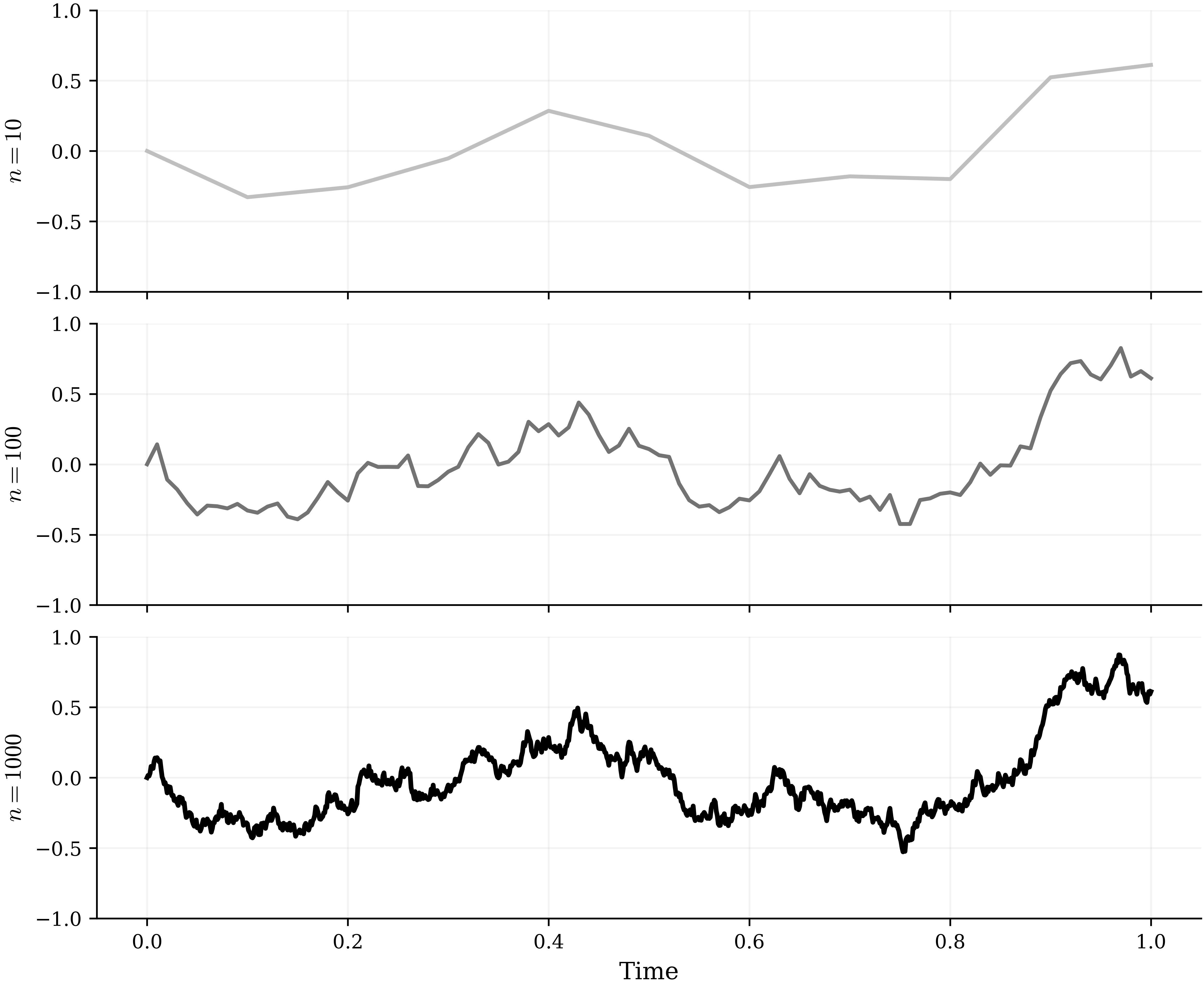
A scaled random walk viewed at increasing resolutions, approaching Brownian motion — Figure 1: A single realization of a scaled random walk viewed at increasing resolutions. As the number of steps increases and each increment is scaled by 1/√n, the path approaches continuous Brownian motion.

As $n$ goes to infinity, the discrete steps blur. The Central Limit Theorem states that because the position is the sum of many independent steps, the distribution of $W^{(n)}(t)$ at any time $t$ converges to a normal distribution with mean zero and variance $t$ [4]:

W^{(n)}(t) \xrightarrow{d} N(0, t) \quad \text{as } n \to \infty

The Central Limit Theorem explains the Gaussian behavior at each fixed time. Extending this convergence to entire sample paths requires a deeper result, known as Donsker's Invariance Principle, which establishes that the scaled random walk converges to Brownian motion as a stochastic process [4].

This limiting process behaves in a way that standard calculus cannot easily describe. In 1909, the French physicist Jean Perrin observed microscopic pollen grains suspended in water and noted that their random paths had no defined velocity [3]. Mathematically, these limiting paths are continuous everywhere but differentiable nowhere. Because the path is made of infinitely many tiny, independent shocks, zooming in on any section reveals more jaggedness rather than a flat line. There are no smooth curves, which means we can never draw a tangent line. The instantaneous speed, the derivative of the path with respect to time, does not exist.

A Preview of Stochastic Calculus

Remarkably, despite this roughness, Brownian paths possess a well-defined quadratic variation. This seemingly paradoxical property becomes the foundation of Itô calculus and much of modern quantitative finance.

Now we have a continuous noise engine that does not explode. The next step is to define its rules so the speculator can use it.

Defining Standard Brownian Motion

We call this continuous limit standard Brownian motion, represented by $W(t)$ . This process is often called the Wiener process, after Norbert Wiener, who gave its first rigorous mathematical construction in 1923 [5].

A process $W(t)$ is a standard Brownian motion if it satisfies three properties [4]:

It starts at zero: $W(0) = 0$ . The model uses today's price as our baseline.
It has independent increments: increments over disjoint time intervals are mutually independent random variables. Informally, this means that the randomness accumulated over one interval tells us nothing about the randomness accumulated over any later, non-overlapping interval.
It has stationary Gaussian increments: the change over any interval is normally distributed with mean zero and a variance equal to the length of that interval:
$W(t) - W(s) \sim N(0, t - s)$

To understand how the random noise evolves through time, we first need the probability of Brownian motion moving from one value to another over a given time interval. This is described by the transition density function of standard Brownian motion, $p(\tau,x,y)$ [4]:

p(\tau, x, y) = \frac{1}{\sqrt{2\pi\tau}} e^{-\frac{(y-x)^2}{2\tau}}

This density describes the driving noise process $W(t)$ , not the stock price itself. When we later introduce arithmetic Brownian motion, the stock's distribution is obtained by shifting and scaling this Brownian motion through its drift and volatility parameters.

Read this equation as a bell curve that gradually flattens and spreads as time passes. The further into the future we look, the greater the uncertainty becomes.

The Variance of Forecasts

Because the model assumes that variance grows linearly with time, the standard deviation grows with the square root of time, $\sqrt{t}$ [4]. To double the expected range of our forecasting error, we must look four times further into the future. This square-root relation is why short-term projections under the model appear relatively tight, while long-term forecasts quickly become highly uncertain.

In 1900, Louis Bachelier used this process to model stock prices in his doctoral thesis, proposing what is known as arithmetic Brownian motion [1, 2]:

S(t) = S(0) + \alpha t + \sigma W(t)

This model describes the stock price as a balance between two competing forces: a steady, deterministic drift that represents the average long-term growth of the company, and a scaled random noise term that represents market volatility.

Using this model, the speculator can price an option. By simulating thousands of potential paths for $S(t)$ over thirty days, the speculator can compute the option payoff at maturity for each path, average these values, and discount the result back to today. This average converges to the fair option price.

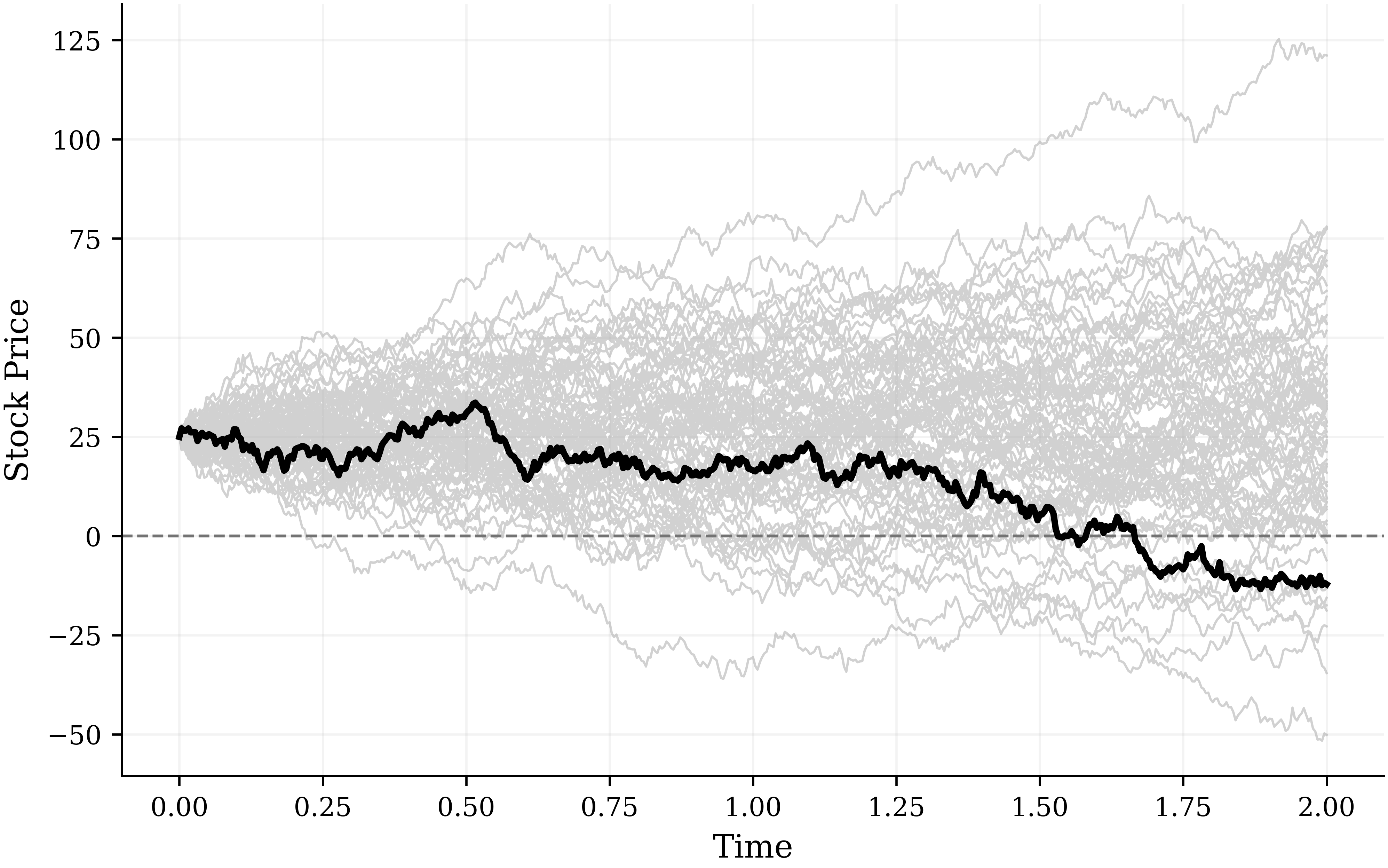
Simulated stock price paths under Arithmetic Brownian Motion crossing below zero — Figure 2: Simulated stock price paths under Arithmetic Brownian Motion. While most trajectories remain positive, the model permits prices to cross below zero over sufficiently long horizons, revealing one of its fundamental limitations.

However, if we examine the simulated paths in Figure 2 closely, a problem appears. If volatility is high or the time horizon is long, some simulated price paths drop below zero.

In the real world, stock prices cannot be negative. Shareholders benefit from limited liability, meaning the worst-case scenario is that the stock price falls to zero. Yet, because Bachelier's model adds absolute dollar changes rather than percentage changes, it treats a stock drop from $10 to $5 as having the same probability as a drop from $500 to $495.

This is a structural flaw. It assigns a positive probability to negative stock prices, which violates the legal reality of equity markets. To resolve this, we need a model where price changes are relative rather than absolute. We need a framework where price movements are modeled as percentage returns, ensuring the price can never fall below zero. This limitation of Bachelier's model motivated the development of Geometric Brownian Motion, where prices can fluctuate infinitely but are naturally bounded by zero.

References

Bachelier, Louis. "Théorie de la Spéculation." Annales Scientifiques de l'École Normale Supérieure 17 (1900): 21–86.
Davis, Mark H. A., and Alison Etheridge. Speculation: Louis Bachelier and the Origins of Modern Finance. Princeton University Press, 2006.
Perrin, Jean. "Mouvement brownien et réalité moléculaire." Annales de Chimie et de Physique 18 (1909): 1–114.
Shreve, Steven E. Stochastic Calculus for Finance II: Continuous-Time Models. Springer, 2004.
Wiener, Norbert. "Differential Space." Journal of Mathematical Physics 2, no. 1–4 (1923): 127–146.